26/09/2024 Tài liệu ôn thi chứng chỉ CFA

Quantitative Methods CFA (Môn Phương pháp phân tích định lượng CFA)

Nội dung chính

Môn Phương pháp phân tích định lượng (Quantitative Methods CFA) là môn học nền tảng có xuất hiện trong Level 1 và 2. Nó tập trung vào cả công thức và khái niệm và mang tính định lượng khá nhiều. Cụ thể môn học này về cái gì và tập trung vào phần kiến thức nào, hãy cùng TACA tìm hiểu nhé!

1. Môn Phương pháp phân tích định lượng trong từng level (Quantitative Methods CFA in 3 levels)

1.1. Trọng số môn Quantitative Methods CFA trong bài thi của các level

Môn Phương pháp phân tích định lượng nhìn sơ qua có thể thấy nó có tỷ trọng và lượng câu hỏi không quá cao chỉ ở khoảng 5-10% nhưng số lượng công thức thì tới khoảng 150, là rất nhiều so với tỷ trọng môn học. Vậy bạn có thể biết được môn học này mang tính định lượng cao và cần sử dụng máy tính nhiều. Hãy luyện tập sử dụng máy tính, làm bài tập tính toán nhiều ở môn học này.

Level	Tỷ trọng	Số lượng câu hỏi	Số lượng công thức
Level 1	6-9%	Khoảng 16	Khoảng 100
Level 2	5-10%	Khoảng 4-8	Khoảng 50
Level 3	0	0	0

1.2. Chi tiết nội dung học của môn Quantitative Methods CFA trong các level

Quantitative Methods CFA Level 1

Ở Level 1, Viện CFA đưa ra 11 mô-đun cho môn Phân tích phương pháp định lượng (Quantitative Methods CFA):

STT	Mô-đun môn học	Mô tả
1	Tỷ suất và lợi nhuận (Rates and Returns)	Hiểu lãi suất như là tỷ suất lợi nhuận yêu cầu, lãi suất chiết khấu hoặc chi phí cơ hội, và giải thích lãi suất là tổng của lãi suất thực không rủi ro và các phí bảo hiểm bù đắp cho nhà đầu tư khi chịu các loại rủi ro khác nhau. Tính toán và giải thích các phương pháp khác nhau để đo lường lợi nhuận theo thời gian và mô tả các ứng dụng phù hợp của chúng. So sánh tỷ suất lợi nhuận theo trọng số tiền và theo trọng số thời gian, và đánh giá hiệu suất của danh mục đầu tư dựa trên các thước đo này. Tính toán và giải thích các thước đo lợi nhuận hàng năm và lợi nhuận lãi kép liên tục, và mô tả các ứng dụng phù hợp của chúng. Tính toán và giải thích các thước đo lợi nhuận chính và mô tả các ứng dụng phù hợp của chúng.
2	Giá trị thời gian của tiền trong tài chính (Time Value of Money in Finance)	Tính toán và giải thích giá trị hiện tại (PV) của các công cụ thu nhập cố định và cổ phiếu dựa trên dòng tiền dự kiến trong tương lai. Tính toán và giải thích lợi suất ngầm của các công cụ thu nhập cố định và lợi suất yêu cầu và tăng trưởng ngầm của các công cụ cổ phiếu, dựa trên giá trị hiện tại (PV) và dòng tiền. Giải thích nguyên tắc cộng tính dòng tiền, tầm quan trọng của nó đối với điều kiện không có cơ hội kiếm lời miễn phí, và việc sử dụng nó để tính toán lãi suất kỳ hạn ngầm, tỷ giá hối đoái kỳ hạn và giá trị quyền chọn.
3	Các thước đo thống kê về lợi nhuận tài sản. (Statistical Measures of Asset Returns)	Tính toán, giải thích và đánh giá các thước đo xu hướng trung tâm và vị trí để giải quyết một vấn đề đầu tư. Tính toán, giải thích và đánh giá các thước đo độ phân tán để giải quyết một vấn đề đầu tư. Giải thích và đánh giá các thước đo độ lệch và độ nhọn để giải quyết một vấn đề đầu tư. Giải thích mối tương quan giữa hai biến số để giải quyết một vấn đề đầu tư.
4	Cây xác suất và kỳ vọng có điều kiện (Probability Trees and Conditional Expectations)	Tính giá trị kỳ vọng, phương sai và độ lệch chuẩn, đồng thời minh họa ứng dụng của chúng vào các vấn đề đầu tư. Biểu diễn một vấn đề đầu tư dưới dạng cây xác suất và giải thích việc sử dụng kỳ vọng có điều kiện trong ứng dụng đầu tư. Tính và giải thích xác suất cập nhật trong một bối cảnh đầu tư bằng công thức Bayes.
5	Toán học danh mục đầu tư (Portfolio Mathematics)	Tính toán và giải thích giá trị kỳ vọng, phương sai, độ lệch chuẩn, hiệp phương sai và tương quan của lợi suất danh mục đầu tư. Tính toán và giải thích hiệp phương sai và tương quan của lợi suất danh mục đầu tư bằng cách sử dụng hàm xác suất liên hợp cho lợi suất. Định nghĩa rủi ro thiếu hụt, tính toán tỷ lệ an toàn đầu tiên và xác định danh mục đầu tư tối ưu bằng tiêu chí an toàn đầu tiên của Roy.
6	Phương pháp mô phỏng (Simulation Methods)	Giải thích mối quan hệ giữa phân phối chuẩn và phân phối lognormal, và lý do tại sao phân phối lognormal được sử dụng để mô hình hóa giá tài sản khi sử dụng lợi suất tài sản ghép liên tục. Mô tả mô phỏng Monte Carlo và giải thích cách nó có thể được sử dụng trong các ứng dụng đầu tư. Mô tả việc sử dụng lấy mẫu bootstrap trong việc thực hiện một mô phỏng dựa trên dữ liệu quan sát trong các ứng dụng đầu tư.
7	Ước lượng và suy luận (Estimation and Inference)	So sánh và đối chiếu lấy mẫu ngẫu nhiên đơn giản, lấy mẫu ngẫu nhiên phân tầng, lấy mẫu cụm, lấy mẫu thuận tiện và lấy mẫu theo đánh giá, cũng như tác động của chúng đối với lỗi lấy mẫu trong một vấn đề đầu tư. Giải thích định lý giới hạn trung tâm và tầm quan trọng của nó đối với phân phối và sai số chuẩn của trung bình mẫu. Mô tả việc sử dụng lấy mẫu lại (bootstrap, jackknife) để ước tính phân phối lấy mẫu của một thống kê.
8	Kiểm tra giả thuyết (Hypothesis Testing)	Giải thích kiểm định giả thuyết và các thành phần của nó, bao gồm ý nghĩa thống kê, lỗi loại I và loại II, và sức mạnh của một kiểm định Xây dựng các kiểm định giả thuyết và xác định ý nghĩa thống kê của chúng, lỗi loại I và loại II liên quan, và sức mạnh của kiểm định cho một mức ý nghĩa nhất định So sánh và đối chiếu các kiểm định tham số và phi tham số, và mô tả các tình huống mà mỗi loại kiểm định phù hợp hơn
9	Kiểm tra tính độc lập tham số và phi tham số (Parametric and Non-Parametric Tests of Independence)	Giải thích các phép kiểm định tham số và phi tham số của giả thuyết rằng hệ số tương quan của tổng thể bằng không và xác định xem giả thuyết có bị bác bỏ ở mức ý nghĩa cho trước hay không. Giải thích các phép kiểm định độc lập dựa trên dữ liệu bảng liên kết.
10	Hồi quy tuyến tính đơn giản (Simple Linear Regression)	Mô tả mô hình hồi quy tuyến tính đơn giản, cách sử dụng tiêu chí bình phương nhỏ nhất để ước lượng hệ số hồi quy và cách giải thích các hệ số này. Giải thích các giả định cơ bản của mô hình hồi quy tuyến tính đơn giản và mô tả cách dư sai và biểu đồ dư sai cho thấy liệu các giả định này có bị vi phạm hay không. Tính toán và giải thích các thước đo độ vừa vặn, xây dựng và đánh giá các kiểm định độ vừa vặn và của hệ số hồi quy trong hồi quy tuyến tính đơn giản. Mô tả việc sử dụng phân tích phương sai (ANOVA) trong phân tích hồi quy, giải thích kết quả ANOVA và tính toán, giải thích sai số chuẩn của ước lượng trong hồi quy tuyến tính đơn giản. Tính toán và giải thích giá trị dự đoán cho biến phụ thuộc và khoảng dự đoán cho nó, cho trước một mô hình hồi quy tuyến tính ước lượng và một giá trị cho biến độc lập. Mô tả các dạng chức năng khác nhau của hồi quy tuyến tính đơn giản.
11	Giới thiệu về các Kỹ thuật Dữ liệu Lớn (Introduction to Big Data Techniques)	Mô tả các khía cạnh của “fintech” liên quan trực tiếp đến việc thu thập và phân tích dữ liệu tài chính Mô tả dữ liệu lớn, trí tuệ nhân tạo và học máy Mô tả ứng dụng của dữ liệu lớn và khoa học dữ liệu trong quản lý đầu tư

Quantitative Methods CFA Level 2

Phân tích phương pháp định lượng (Quantitative Methods) ở Level 2 có 7 mô-đun:

STT	Mô-đun môn học	Mô tả
1	Các nguyên tắc cơ bản của hồi quy đa biến và các giả định tiềm ẩn (Basics of Multiple Regression and Underlying Assumptions)	Mô tả các loại vấn đề đầu tư được giải quyết bằng hồi quy tuyến tính đa biến và quá trình hồi quy Xây dựng một mô hình hồi quy tuyến tính đa biến, mô tả mối quan hệ giữa biến phụ thuộc và một số biến độc lập, và giải thích các hệ số hồi quy ước lượng Giải thích các giả định cơ bản của một mô hình hồi quy tuyến tính và giải thích các biểu đồ dư sai cho thấy các vi phạm tiềm năng của các giả định này
2	Đánh giá độ phù hợp của mô hình hồi quy (Evaluating Regression Model Fit and Interpreting Model Results)	Đánh giá mức độ phù hợp của một mô hình hồi quy đa biến trong việc giải thích biến phụ thuộc bằng cách phân tích kết quả bảng ANOVA và các thước đo độ phù hợp. Đặt ra giả thuyết về ý nghĩa của hai hoặc nhiều hệ số trong một mô hình hồi quy đa biến và giải thích kết quả của các kiểm định giả thuyết liên hợp. Tính toán và giải thích giá trị dự đoán cho biến phụ thuộc, dựa trên mô hình hồi quy ước lượng và các giá trị giả định của biến độc lập.
3	Mô hình khuyết tật (Model Misspecification)	Mô tả cách sai số mô hình ảnh hưởng đến kết quả của phân tích hồi quy và cách tránh các dạng sai số phổ biến. Giải thích các loại dị phương sai và cách nó ảnh hưởng đến suy luận thống kê. Giải thích tương quan tuần tự và cách nó ảnh hưởng đến suy luận thống kê. Giải thích đa cộng tuyến và cách nó ảnh hưởng đến phân tích hồi quy.
4	Các dạng mở rộng của hồi quy đa biến (Extensions of Multiple Regression)	Mô tả phân tích ảnh hưởng và các phương pháp phát hiện điểm dữ liệu có ảnh hưởng Xây dựng và giải thích một mô hình hồi quy đa biến bao gồm các biến độc lập định tính Xây dựng và giải thích một mô hình hồi quy logistic
5	Phân tích dữ liệu chuỗi thời gian (Time-Series Analysis)	Tính toán và đánh giá giá trị xu hướng dự đoán cho một chuỗi thời gian, được mô hình hóa như một xu hướng tuyến tính hoặc xu hướng logarit-tuyến tính, dựa trên các hệ số xu hướng ước tính. Mô tả các yếu tố quyết định việc sử dụng xu hướng tuyến tính hay logarit-tuyến tính với một chuỗi thời gian cụ thể và đánh giá hạn chế của các mô hình xu hướng. Giải thích yêu cầu về tính dừng của chuỗi thời gian và mô tả ý nghĩa của một chuỗi không dừng. Mô tả cấu trúc của mô hình tự hồi quy (AR) bậc p và tính toán dự báo một và hai kỳ trước dựa trên các hệ số ước tính. Giải thích cách sử dụng tự tương quan của phần dư để kiểm tra xem mô hình tự hồi quy có phù hợp với chuỗi thời gian hay không. Giải thích sự hồi quy trung bình và tính toán mức độ hồi quy trung bình. So sánh dự báo trong mẫu và ngoài mẫu và so sánh độ chính xác dự báo của các mô hình chuỗi thời gian khác nhau dựa trên tiêu chí lỗi bình phương trung bình. Giải thích sự bất ổn của các hệ số của mô hình chuỗi thời gian. Mô tả đặc điểm của quá trình đi bộ ngẫu nhiên và so sánh chúng với quá trình dừng. Mô tả tác động của gốc đơn vị đối với phân tích chuỗi thời gian, giải thích khi nào gốc đơn vị có khả năng xảy ra và cách kiểm tra chúng, và chứng minh cách một chuỗi thời gian có gốc đơn vị có thể được chuyển đổi để phân tích với mô hình AR. Mô tả các bước của kiểm định gốc đơn vị cho tính không dừng và giải thích mối liên hệ của kiểm định với các mô hình chuỗi thời gian tự hồi quy. Giải thích cách kiểm định và điều chỉnh tính mùa vụ trong một mô hình chuỗi thời gian và tính toán, giải thích giá trị dự báo bằng cách sử dụng mô hình AR với độ trễ theo mùa. Giải thích dị phương sai có điều kiện tự hồi quy (ARCH) và mô tả cách các mô hình ARCH có thể được áp dụng để dự đoán phương sai của một chuỗi thời gian. Giải thích cách các biến chuỗi thời gian nên được phân tích về tính không dừng và/hoặc đồng tích trước khi sử dụng trong hồi quy tuyến tính. Xác định một mô hình chuỗi thời gian phù hợp để phân tích một vấn đề đầu tư nhất định và biện minh cho lựa chọn đó.
6	Máy học (Machine Learning)	Mô tả học máy có giám sát, học máy không giám sát và học sâu Mô tả quá trình quá khớp và xác định các phương pháp giải quyết nó Mô tả các thuật toán học máy có giám sát – bao gồm hồi quy có phạt, máy vectơ hỗ trợ, k-láng giềng gần nhất, phân loại và hồi quy cây, học tập tổng thể và rừng ngẫu nhiên – và xác định các vấn đề mà chúng phù hợp nhất Mô tả các thuật toán học máy không giám sát – bao gồm phân tích thành phần chính, phân cụm k-means và phân cụm phân cấp – và xác định các vấn đề mà chúng phù hợp nhất Mô tả mạng thần kinh, mạng học sâu và học tăng cường
7	Dự án dữ liệu lớn (Big Data Projects)	Xác định và giải thích các bước trong một dự án phân tích dữ liệu Mô tả mục tiêu, bước và ví dụ về chuẩn bị và sắp xếp dữ liệu Đánh giá độ phù hợp của một thuật toán học máy Mô tả mục tiêu, phương pháp và ví dụ về khám phá dữ liệu Mô tả các phương pháp trích xuất, chọn lọc và thiết kế đặc trưng từ dữ liệu văn bản Mô tả mục tiêu, bước và kỹ thuật trong đào tạo mô hình Mô tả chuẩn bị, sắp xếp và khám phá dữ liệu dựa trên văn bản cho dự báo tài chính

Xem thêm:

2. Mẫu câu hỏi & đáp án môn Quantitative Methods CFA trong các level

2.1. Câu hỏi Quantitative Methods CFA Level 1

Question 1:

An analyst determines that the probabilities of two events are as follows:

Event	Description	Probability
A	Price of oil increases	0.33
B	S&P 500 Index increases	0.49

Assuming the events are independent but not mutually exclusive, the probability that at least one of the two events will occur is closest to:

0.16
0.66
0.82

Solution:

Quantitative Methods CFA

The probability that at least one of the two events ( A or B) will occur is the same as the probability that:

Only A ( one event ) will occur, or
Only B ( one event ) will occur, or
Both A and B ( two events ) will occur.

The addition rule for probability states that for events that are not mutually exclusive:

P( A or B) = P(A) + P(B) − P(AB)

Note that the probability that both events occur, which is possible since the events are not mutually exclusive, must be subtracted to avoid double counting that probability.

In this scenario, P(A) and P(B) are given, but the probability of both A and B [ P( AB) ] is not given. However, for independent events, P(AB) can be calculated according to the multiplication rule for probability as P(A) P(B). Substituting P(A) P(B) for P(AB) into the addition rule above:

P(A or B) = P(A) + P(B) − P(A) P(B)

= 0.33 + 0.49 − (0.33 × 0.49)

= 0.6583 ≈ 0.66, or 66%

(Choice A) 0.1617 is the result of multiplying P(A) and P(B). This is P(AB), the probability that both A and B will occur, not the probability of A or B.

(Choice C) 0.8200 is the result of treating A and B as mutually exclusive and not subtracting the probability that both events will occur, P(AB). This has the effect of double-counting the probability of A and B both occurring and so overestimates the probability of A or B occurring.

Things to remember:
The addition rule for probability states that for two events that are not mutually exclusive, such as A and B in this scenario, P(A or B) = P(A) + P(B) − P(AB). For independent events, the multiplication rule for probability states that P(AB) = P(A) P(B).

Question 2:

A researcher formulates a null hypothesis stating that a country’s average inflation is 2%. After testing a sample, the researcher fails to reject the null hypothesis when the actual average inflation is not 2%. This most likely results in a:

Type I error.
Type II error.
correct decision.

Solution:

	Actual Situation
Decision from statistical test	Null (H₀) is true	Null (H₀) is false
Do not reject null (H₀)	Correct decision	Type II error
Reject null (H₀), accept alternative (H_a)	Type I error	Correct decision

Hypothesis testing involves a decision regarding whether to reject a null hypothesis (H0) based on statistical tests. In this question, the null hypothesis states that the country’s average inflation is 2% (H₀: μ = 2%). Conversely, the alternative hypothesis states that the country’s average inflation is not 2% (H_a: μ ≠ 2%).

There are two types of errors that can result from the decision to reject or to not reject the null hypothesis:

Type I error: Rejecting the null hypothesis when it is true
Type II error: Failing to reject the null hypothesis when it is false

Here, the null hypothesis is false since actual average inflation is not 2%. Failing to reject the false null hypothesis in this case results in a Type II error.

(Choice A) A Type I error results from rejecting a null hypothesis when it is true. An example of a Type I error would be the analyst rejecting the null hypothesis (H₀: μ = 2%) when the actual average inflation is 2%.

(Choice C) Given the actual situation that the average inflation is not 2% (ie, the null hypothesis is false), the correct decision is to reject the null hypothesis (H₀: μ = 2%).

Things to remember:
A Type I error results from rejecting the null hypothesis when it is true. A Type II error results from failing to reject the null hypothesis when it is false.

2.2. Câu hỏi Quantitative Methods CFA Level 2

Passage:

Jae Park, CFA, is a manager of a hedge fund that bases its security selection on advanced quantitative analysis. For several open job positions with the fund, Park is looking to hire people with scientific and research backgrounds. Using multiple regression, she would like to evaluate the relationship between the expected salary of the candidates based on their years of experience (EXP), number of published research papers (PRP), and amount of grant funding received in their career (GF). The results of that regression are shown below, along with sample critical values. Park wishes to test the results at a 5% significance level (α = 0.05).

Quantitative Methods CFA

Park also notices that each candidate attended one of five universities. She is considering how to add a variable for university attended to the regression model and believes dummy variables are the best way to capture this.

Finally, Park suspects that her regression in its current form may violate regression assumptions. Her concern is that her model might have an artificially large R² and t-statistics that are understated.

Question 1:

Based on the data in Exhibit 1, the regression is most likely a good predictor of projected salary since:

it has a high R ²
the F – statistic has a low p – value.
most coefficients are statistically significant.

Solution:

ANOVA Data	df	Sum of Squares (SS)	Mean SS	F	Significance F
Regression (k )	3	30,430.34	10,143.40	18.643	0
Residual (n – k – 1 )	22	11,969.66	544.08
Total	25	42,400.00
Observations	26
R ²	0.718
Standard error	23.325

Quantitative Methods CFA

Hypothesis testing verifies whether a regression is a good predictor of the dependent variable. Testing can be performed on coefficients or the overall regression.

The F-statistic is used to test whether the overall regression (ie, the combination of all slope coefficients) is statistically significant. The null hypothesis (H₀) states that the model has no statistically significant coefficients, while the alternative hypothesis (H_a) states that at least one coefficient is significant.

The ANOVA table provides the F – statistic’s p-value ( labeled “significance F ” ). H₀ is rejected if the p – value is less than the level of significance (α). In this scenario, the p – value is less than α (0 < 0.05), so H₀ is rejected and the regression is statistically significant. In other words, the regression is a good predictor of the dependent variable.

(Choice A) R² gauges how closely the data fit the regression line. Adding independent variables will increase R², even if those variables are only slightly correlated with the dependent variable. Furthermore, R² does not measure statistical significance. Models may have multiple coefficients without statistical significance and still have a high R². The model’s predictive power depends mainly on the statistical significance of the regression and the coefficients.

(Choice C) A t– test can determine if a slope coefficient is statistically significant. However, the model’s overall fit cannot be determined from t– tests due to possible interactions among the independent variables. Individual coefficients can be statistically significant, but the overall regression is not.

Things to remember:
The F– statistic is used to test how well the regression explains the dependent variable. The null hypothesis H₀ states that none of the coefficients are statistically significant, and it can be rejected if the p – value of the F – statistic is less than α. Rejecting H₀ indicates that the model is a statistically significant predictor of the dependent variable.

Question 2:

According to Exhibit 1, the most appropriate interpretation of the coefficients is that a higher expected salary will result from:

more published papers and less grant funding.
more published papers and more grant funding.
fewer published papers and more grant funding.

Solution:

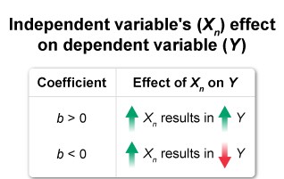
The predicted value of the dependent variable can be derived using the relationship expressed in the regression equation. The slope coefficients of the equation explain the change in the dependent variable, given a one-unit change to one of the independent variables.

The sign of the coefficient indicates the direction of the change in the dependent variable. If the sign of the coefficient is:

positive, then the independent and dependent variables will move in the same direction.
negative, then the independent and dependent variables will move in opposite directions.

In this scenario, the PRP and GF coefficients determine how changes to those variables affect the expected salary:

The PRP coefficient is negative, so a higher PRP variable results in a lower projected salary (Choice A).
The GF coefficient is positive, so a higher GF variable results in a higher projected salary (Choice B).

Thus, a higher salary would be expected from fewer published papers and more grant funding.

Things to remember:
The sign of a slope coefficient indicates how a change in an independent variable affects the dependent variable. If a coefficient has a positive sign, then the independent and dependent variables move in the same direction. If a coefficient has a negative sign, then the independent and dependent variables move in opposite directions.

Question 3:

Based on Exhibits 1 and 2, which slope coefficient is most likely to be statistically significant?

Solution:

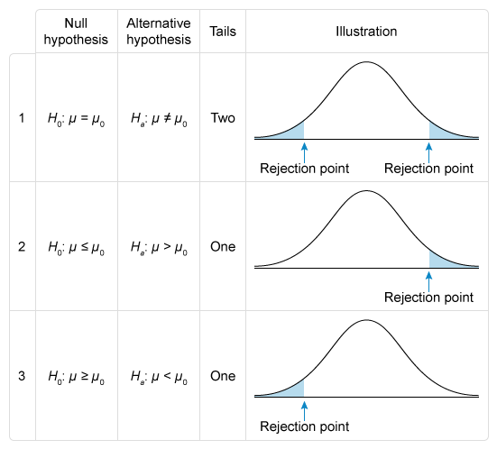
In a regression model, the slope coefficients describe how a change in an independent variable affects the dependent variable. A t– test is used to verify whether a coefficient meaningfully describes the relationship between an independent and dependent variable.

The test seeks to determine whether a coefficient is statistically different from zero. The null hypothesis (H₀) states that the coefficient equals zero, while the alternative hypothesis (H_a) states that the coefficient is not equal to zero. The test is also two-tailed, as shown in the image above.

The test compares the t– statistic (t) to the critical value (t_c), and the null is rejected if the absolute value of the t– statistic is greater than the critical value (ie, reject H₀ if |t| > t_c). Rejection of H₀ means that the coefficient is statistically different from zero (ie, statistically significant).

The steps for the t– test on each of the coefficients are as follows:

Steps	Calculations
Solve for the residuals’ degrees of freedom	df = n – k – 1 = 26 – 3 – 1 = 22
Solve for the critical t – value	Critical value for 2-tailed test, df = 22, and 5% significance = 2.0739
Compare each t – statistic to the critical value; reject H0 if \|t \| > t_c	EXP: \|4.550\| > 2.0739; reject H₀ PRP: \|-0.438 \| < 2.0739; cannot reject H₀ GF: \|1.552 \| < 2.0739; cannot reject H₀

Xem thêm:

[Cập nhật] Bóc trần cấu trúc đề thi CFA: Đừng bỏ lỡ bất kỳ điểm nào!

Bài tập Quantitatives Methods CFA (Môn Phương pháp định lượng CFA) kèm đáp án

3. Một số mẹo học và ôn thi môn Quantitative Methods CFA

Hãy tạo một nền tảng vững chắc: Vì trong xuyên suốt chương trình học CFA, môn Phương pháp phân tích định lượng mà có các phần kiến thức rải rác, liên quan đến mọi môn học. Nó là những kiến thức cơ bản mà bạn cần nghiên cứu, đào sâu.
Làm bài tập thực hành và lặp đi lặp lại nhiều lần: Viện CFA đề cao tầm quan trọng của việc thực hành, đặc biệt là phần CFA định lượng. Việc trả lời càng nhiều câu hỏi càng tốt có thể hỗ trợ đáng kể cho việc nắm bắt các khái niệm và định dạng kiểm tra của kỳ thi. Đặc biệt là môn học này là môn học thiên về tính toán nhiều hơn nên việc luyện tập là điều quan trọng.
Bắt đầu học Phương pháp định lượng càng sớm càng tốt: Thứ tự học các môn học là câu hỏi thường gặp với hầu hết các ứng viên. Tốt nhất là bạn nên bắt đầu với Phương pháp định lượng. Các mô đun môn học này giới thiệu các khái niệm cơ bản tạo nên chương trình dạy ở Level 1. Ngoài ra, khi bạn học tới các Level sau thì bạn sẽ nhận ra nội dung môn học này sẽ lặp lại trong suốt chương trình ở mọi Level.
Ưu tiên học bản chất, cách hình thành công thức hơn là ghi nhớ công thức một cách đơn thuần: Bạn có thể sử dụng máy tính khá nhiều trong môn học này, tuy nhiên việc thành thạo nội dung này không chỉ liên quan đến viện tính toán các con số. Mặc dù việc áp dụng các khái niệm là quan trọng nhưng sẽ dễ nhớ lại cách thực hiện hơn nếu bạn thực sự hiểu ngữ cảnh, cách nó được áp dụng và hình thành nên. Trong một số trường hợp, nếu bạn thực sự hiểu các khái niệm, bạn sẽ không phải dựa vào máy tính của mình chút nào.
Level 2 có nhiều khái niệm, lý thuyết hơn Level 1 nhưng bạn vẫn phải tính toán: Phương pháp định lượng cấp độ 2 phức tạp hơn: nhiều mô hình phức tạp hơn, nhiều biến số hơn, nhiều công thức hơn, nhưng cũng nhiều lý thuyết và hiểu biết hơn về lý do tại sao toán học hoạt động. Nhưng bạn vẫn phải tính toán các con số.
Hãy chắc chắn rằng bạn thành thạo các chức năng của máy tính: Bạn cần cố gắng luyện tập thật nhiều cách bấm máy cho các dạng câu hỏi khác nhau. Đừng để vào phòng thi rồi mới hối hận vì không học cách bấm máy sớm hơn. Máy tính sẽ giúp bạn tiết kiệm rất nhiều thời gian, tránh được việc loay hoay với cả dãy số liệu. Và dù sao đi nữa đây cũng là một ký năng cần thiết cho một dân tài chính, kế toán. Bạn có thể xem thêm hướng dẫn sử dụng máy tính BA II Plus Professional hoặc HP 12C ở các website chính thức của nhà cung cấp máy tính.

Câu hỏi thường gặp

Tổng quan về Phương pháp phân tích định lượng (Quantitative Methods CFA)

Phân tích báo cáo tài chính (Quantitive Methods CFA) đưa ra những khái niệm cơ bản trong quá trình phân tích và định giá như: Giá trị thời gian của tiền tệ; NPV; IRR; Khái niệm về xác suất, thống kê; Kiểm định giả thuyết và Phân tích kỹ thuật. Quantitative Methods là tiền đề để học các môn học CFA khác như: Financial Reporting and Analysis, Corporate Finance, Equity Investment, Fixed Income, và đặc biệt là Portfolio Management and Wealth Planning.

Môn Phương pháp phân tích định lượng (Quantitative Methods CFA) có khó không?

Phương pháp phân tích định lượng là một trong những chủ đề khó nhất trong chương trình giảng dạy CFA Cấp độ 1 và Cấp độ 2, vì nó thường ít quen thuộc nhất. Các ứng viên chưa tiếp xúc nhiều với các kỹ thuật và khái niệm định lượng có thể gặp khó khăn hơn với chủ đề này.

Nên học môn Phương pháp phân tích định lượng (Quantitative Methods CFA) như thế nào?

Phần môn học này là phần dựa trên công thức và toán học nhiều nhất. Nó cũng quan trọng trong kỳ thi CFA ở hai cấp độ đầu tiên, chiếm 12% kỳ thi ở Level 1 và 5-10% kỳ thi Level 2. Nhưng kiến thức thực sự được áp dụng vào tất cả các phần của chương trình giảng dạy, vì vậy các ứng viên phải hiểu các nguyên tắc cơ bản của Phương pháp định lượng ở Level 1. Mọi người học các ý tưởng định lượng theo cách khác nhau, nhưng tốt nhất là luôn thực hành, thực hành, thực hành.

Nếu bạn đang cần tư vấn về lộ trình học và ôn tập CFA, đừng ngần ngại liên lạc với Taca Academy!